How to detect a hologram with OpenCV

Holographic print detection is an essential task in applications requiring automatic validation of government-issued ids, banknotes, credit cards and other printed documents from a video stream. Today we’ll discuss how to approach this problem with Python and OpenCV.

Unique features of holographic print

Human can instantly recognize a holographic print by two main characteristics:

  • highly reflective
  • color changes within a wide range depending on relative position of the light source
Sample image from Google

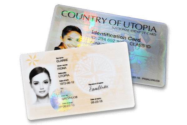
Some prints, like logos on credit cards, may have more advanced security features when holographic print incorporates specific sequence of images which is ‘played’ when you rotate it against the light source. In this article, we will focus on just two main characteristics above.

Sample data

First, we’ll need to collect the data for analysis – a sequence of frames capturing the holographic print from different angles under directional light source. The optimal way to achieve this is to record a video with a smartphone with torch turned on, like this:

Now, as we have the data to experiment, what’s our plan?

  1. Perform segmentation – accurately detect the zone of interest on each frame
  2. Unwarp and stack zone of interest pixels in a way ensuring coordinates match between frames
  3. Analyze resulting data structure to find coordinates of hologram’s pixels
  4. Display results

Image segmentation

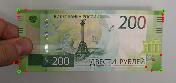
Because the object which have holographic print on it (or a camera) will be moving, we’ll need to detect the initial position and track it throughout the frame sequence. In this case, a banknote has a rectangular shape. Let’s start by identifying the biggest rectangle on the image.

# convert to grayscale
gray = cv2.cvtColor(img, cv2.COLOR_BGR2GRAY)
# get corners
features = cv2.goodFeaturesToTrack(gray, 500, 0.01, 10)
corners = features.squeeze()
# get some number of corners closest to corresponding frame corners
corner_candidates = list(map(lambda p: closest(corners, p[0], p[1], HoloDetector.NUM_CANDIDATES),
                             ((0, 0), (0, gray.shape[0]), (gray.shape[1], gray.shape[0]), (gray.shape[1], 0))))
# check for rectangularity and get a maximum area rectangle
combs = itertools.product(*corner_candidates)
max_rect = None
max_area = 0
for c1, c2, c3, c4 in combs:
    # calculate angles using
    angles = [angle(c1 - c2, c3 - c2),
              angle(c2 - c3, c4 - c3),
              angle(c1 - c4, c3 - c4)]
    if np.allclose(angles, np.pi / 2, rtol=0.05):
        area = la.norm(c2 - c1) * la.norm(c3 - c2)
        if area > max_area:
            max_rect = [c1, c2, c3, c4]
            max_area = area

Here, goodFeaturesToTrack function is used to get strong corners from the image, then maximum rectangle of a proper orientation is estimated.

Tracking the movement

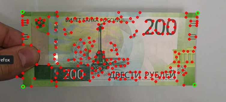
An obvious way to track the movement would be to detect corners in a similar way on all consecutive frames, however, this method is not robust to changes in the background and severe rotations of the object. Instead, we will detect initial features inside the rectangle, and estimate their new positions on consecutive frames using optical flow algorithm

# get start keypoints inside rectangle
features = cv2.goodFeaturesToTrack(gray, 1000, 0.01, 19)
rect_contour = np.array(rect).astype(np.int32)
# take only points inside rectangle area
last_features = np.array(list(filter(lambda p: cv2.pointPolygonTest(rect_contour, tuple(p.squeeze()), False), features)))

Note: we could skip rectangle detection altogether and detect keypoints on full image, but it’s unrealistic to have such a convenient neutral background in a real-world scenario.

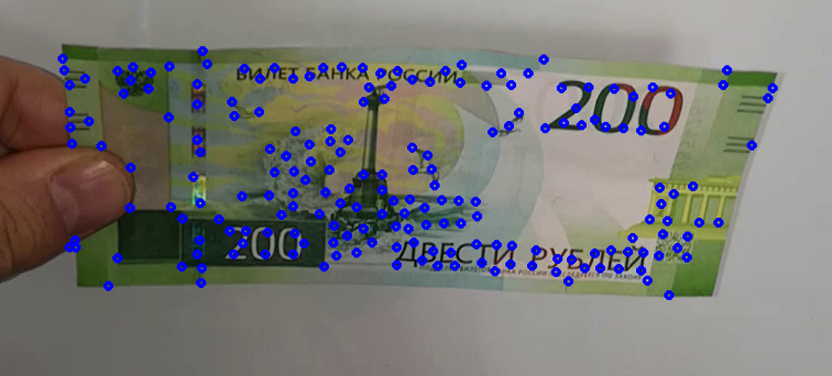
Now it’s possible to look for same keypoints on every next frame using a function which implements Lucas-Kanade method. Additional trick here is to filter out unstable keypoints by running an algorithm forward and backwards, and then cross-checking result with known initial keypoints.

def checkedTrace(img0, img1, p0, back_threshold=1.0):
    p1, _st, _err = cv2.calcOpticalFlowPyrLK(img0, img1, p0, None, lk_params)
    p0r, _st, _err = cv2.calcOpticalFlowPyrLK(img1, img0, p1, None, lk_params)
    d = abs(p0 - p0r).reshape(-1, 2).max(-1)
    status = d < back_threshold
    return p1, status

# calculate optical flow with cross check
features, status = HoloDetector.checkedTrace(last_gray, gray, last_features)
# filter only cross-checked features
last_features = last_features[status]
features = features[status]

To map pixel coordinates of a given frame to source frame’s coordinates, we’ll need to estimate a transformation matrix with findHomography function, which takes two lists of source and destination keypoints and returns a transformation matrix.

# estimate transformation matrix
m, mask = cv2.findHomography(features, last_features, cv2.RANSAC, 10.0)
# unwarp image into original image coordinates
unwarped = img.copy()
unwarped = cv2.warpPerspective(unwarped, m, img.shape[:2][::-1], flags=cv2.INTER_LINEAR)

Here’s how the video looks after unwarping. Not perfectly aligned, because banknote have some curvature of itself, but much better!

Detecting a hologram

Previous processing steps allowed us to get a data structure like this:

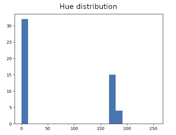
Where z-axis represents the number of frame in the sequence. Let’s create histograms of individual pixel values in HSV color space.

HSV space

As you can see, Hue value have much wider range for pixels of the hologram. Let’s filter pixels based on that and highlight the ones with 5% – 95% percentile range above a certain threshold. Let’s also cutoff dark pixels with too low S and V values.

# quantile range for holo pixels on H component is expected to be much wider
qr = np.quantile(holo_stack[:, :, 0, :], q=0.95, axis=2) - np.quantile(holo_stack[:, :, 0, :], q=0.05, axis=2)
# Saturation and Value thresholds because on lower values H component may be unstable
ms = np.mean(holo_stack[:, :, 1, :], axis=2)
mv = np.mean(holo_stack[:, :, 2, :], axis=2)
filtered_points = []
holo_points = np.where((ms > 50) & (mv > 50) & (qr > HoloDetector.HOLO_THRESHOLD))
holo_mask[tuple(zip(*filtered_points))] = (0, 255, 0)

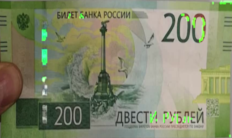
Success! The holograms most visible on the video are highlighted, but we have some false positives. What’s wrong with these pixels?

That is the result of inaccurate unwarping, pixels laying on strong edges have two distinct values. The difference with hologram pixels is that they are not taking all the values in between of these histogram peaks. In other words, their distribution is less uniform. We can use Chi-squared test to check for uniformity and filter these pixels out:

filtered_points = []
# filter detected pixels by uniformity of their distribution, holo points are taking multiple colors,
# while misaligned edge pixels will have only few different values
for y, x in zip(*holo_points):
    freq = np.histogram(self.holo_stack[y, x, 0, :], bins=20, range=(0, 255))[0]
    # checks for uniformity without expected frequencies parameter
    chi, _ = scipy.stats.chisquare(freq)
    if chi < HoloDetector.UNIFORMITY_THRESHOLD:
        filtered_points.append((y, x))
# highlight pixels on mask
self.holo_mask[tuple(zip(*filtered_points))] = (0, 255, 0)

Much better now! Here’s how it looks overlayed on original video:

Two top pieces are highlighted, and the bottom ones, which look more like a foil on this video, aren’t. Another sample with a credit card having a better hologram:

That’s it. See full code on my github. Thanks for reading!

Robust logo detection with OpenCV

With various flavors of convolutional neural nets being all the rage for image processing, one may undeservedly forget about a family of advanced classical algorithms for image classification and object detection. These are SIFT, SURF, (A)KAZE and ORB, with latter one being the popular choice, because it’s:

  • Rotation and scale invariant. Most widely used neural net architectures aren’t.
  • Fast. Able to run at 30+ FPS on a single desktop CPU core with 0.3 MP frames.
  • Free. Some other algorithms, like SIFT and SURF, are patented and require licensing for commercial use.
  • Robust. Able to extract usable features from a single sample image.

Let’s look at ORB from engineering perspective, without re-citing the wikipedia and papers on the algorithm. Suppose we want to detect a DELL logo (completely random choice) on the input image:

First, we need to initialize the detector and set parameters:

 def createDetector():
    detector = cv2.ORB_create(nfeatures=2000)
    return detector

One of a few parameters which can be experimented with without digging deeply into the algorithm implementation is nfeatures – a maximum number of resulting feature vectors detector will estimate. It worth slightly increasing it above the default value of 500. Some additional info on ORB parameters can be found here and here.

Next, let’s define a function to get keypoint coordinates and descriptor vectors from the image:

def getFeatures(img):
    gray = cv2.cvtColor(img, cv2.COLOR_BGR2GRAY)
    detector = createDetector()
    kps, descs = detector.detectAndCompute(gray, None)
    return kps, descs, img.shape[:2][::-1]

The next step is to search for a bounding box of our logo on a query image, here’s how to do it (see comments):

def detectFeatures(img, train_features):
    train_kps, train_descs, shape = train_features
    # get features from input image
    kps, descs, _ = getFeatures(img)
    # check if keypoints are extracted
    if not kps:
        return None
    # now we need to find matching keypoints in two sets of descriptors (from sample image, and from current image)
    # knnMatch uses k-nearest neighbors algorithm for that
    bf = cv2.BFMatcher(cv2.NORM_HAMMING)
    matches = bf.knnMatch(train_descs, descs, k=2)

    good = []
    # apply ratio test to matches of each keypoint
    # idea is if train KP have a matching KP on image, it will be much closer than next closest non-matching KP,
    # otherwise, all KPs will be almost equally far
    for m, n in matches:
        if m.distance < 0.8 * n.distance:
            good.append([m])

    # stop if we didn't find enough matching keypoints
    if len(good) < 0.1 * len(train_kps):
        return None

    # estimate a transformation matrix which maps keypoints from train image coordinates to sample image
    src_pts = np.float32([train_kps[m[0].queryIdx].pt for m in good
                          ]).reshape(-1, 1, 2)
    dst_pts = np.float32([kps[m[0].trainIdx].pt for m in good
                          ]).reshape(-1, 1, 2)

    m, mask = cv2.findHomography(src_pts, dst_pts, cv2.RANSAC, 5.0)

    if m is not None:
        # apply perspective transform to train image corners to get a bounding box coordinates on a sample image
        scene_points = cv2.perspectiveTransform(np.float32([(0, 0), (0, shape[0] - 1), (shape[1] - 1, shape[0] - 1), (shape[1] - 1, 0)]).reshape(-1, 1, 2), m)
        rect = cv2.minAreaRect(scene_points)
        # check resulting rect ratio knowing we have almost square train image
        if rect[1][1] > 0 and 0.8 < (rect[1][0] / rect[1][1]) < 1.2:
            return rect
    return None

Now, to search for a logo on image, we just need to call these functions and visualize result:

# get train features
img = cv2.imread('logo_train.png')
train_features = features.getFeatures(img)
# detect features on test image
region = features.detectFeatures(frame, train_features)
if region is not None:
    # draw rotated bounding box
    box = cv2.boxPoints(region)
    box = np.int0(box)
    cv2.drawContours(img, [box], 0, (0, 255, 0), 2)
# display the image
cv2.imshow("Preview", img)

Here’s how it works for a test image with slight distortion and rotation:

Full code processing images from camera is available on github.

To improve this basic implementation of image detector, you might want to adjust some parameters, add Kalman filter for stabilization, create a more robust set of features using multiple training images, etc. Hope this will help you to start!

Tesseract OCR best practices

Tesseract is an open-source cross-platform OCR engine initially developed by Hewlett Packard, but currently supported by Google. In this post, I want to share some useful tips regarding how to get maximum performance out of it. I won’t cover the basics which can be found in official docs.

0. Know your data

The top most important tip for any data processing task, and OCR is not an exception. Is your OCR suddenly works terrible on production? Is test performance low? Check what images you’re passing to the engine. No, seriously. If you’re looking into low OCR performance issue, first thing dump the image right before OCR engine call and make sure it’s not cropped, distorted, have wrong channel order, etc.

1. Configure parameters

Now to actual Tesseract-related tips. Here’s the list of most important Tesseract parameters:

  • Trained data. On the moment of writing, tesseract-ocr-eng APT package for Ubuntu 18.10 has terrible out of the box performance, likely because of corrupt training data. Download data file separately here and add --tessdata-dir parameter when calling the engine from console.
  • Page Segmentation Mode (--psm). That affects how Tesseract splits image in lines of text and words. Pick the one which works best for you.

Automatic mode is much slower than more specific ones, and may affect performance. Sometimes, it’s feasible to implement a simple domain-specific field extraction pipeline and combine it with Single Line (7) or Single Word (8) page segmentation mode.

  • Engine Mode (--oem). Tesseract has several engine modes with different performance and speed. Tesseract 4 have introduced additional LSTM neural net mode, which often works best. Unfortunately, there’s no LSTM support on Android fork yet.
  • Character whitelist (-c tessedit_char_whitelist="XYZ"). In version 4, whitelists are supported only in legacy engine mode (--oem 0).

Here’s a sample grayscale image with corresponding Tesseract executable call:

tesseract --tessdata-dir . driving_licence.png stdout --oem 3 --psm 7

2. Correct the skew

Tesseract usually successfully corrects skew up to 5 degrees. However, it’s best to correct image rotation before passing it to OCR.

3. Don’t crop the image too close

Tesseract expects the image to have some empty fields (of a background color) around text. That’s rarely the case when text areas are extracted automatically and you may wonder why OCR performance is so bad. To fix that, just pad the images with background color on 20% of text line height. Let’s see how cropping will affect OCR of the image above:

It still looks perfectly readable, but here is what we get when trying to OCR it:

4. Postprocess OCR results

Consider OCR output to be raw data. To get good results, you still need to implement assumptions and knowledge of the specific problem domain.

  • Numeric and text fields. If you expect the field or a single “word” to have either digits or letters, apply right substitution for ambiguous characters. These are most common:
5 → S 1 → I 0 → O
2 → Z 4→ A 8 → B
  • Dictionary words. For text which is expected to consist of dictionary words, perform dictionary checks within some low edit distance, or use a spell checking library. Despite that Tesseract have this functionality built-in, it often didn’t work as expected for me.
  • Punctuation. Characters like -.,;are hard for OCR. If, say, you need to parse a date, consider you don’t have them. Use regular expression, like this: [0-9]{2}[-\\. ]{1,2}[0-9]{2}[-\\. ]{1,2}(19|20)[0-9]{2}

Finally, refer to Tesseract performance guide for more ideas. Good luck!

How to use RS256 tokens with Flask-JWT

As a follow-up of my previous post on JWT authentication in Flask, I want to discuss the implications of using RS256 algorithm for signing the tokens with Flask-JWT library. First of all, what’s the difference between RS256 and HS256 (a standard one) algorithms for JWT?

  • HS256 stands for HMAC with SHA-256. That’s an algorithm which encrypts and hashes the message (a JSON data in our case) at the same time using symmetrical secret key. The same key is used for encryption and decryption of the message.
  • RS256 is an RSA encryption plus SHA-256 hashing. RSA is an asymmetric encryption algorithm, which means it operates on a pair of keys – public and private. Private key is used to encrypt a token, and public one – to decipher it. You can share the public key freely without compromising authentication scheme.

In a simple case, there might be no need to use RS256. However, if you want to validate tokens on client for any reason, for example, to protect against MITM attack (especially in case of no transport-level security), or to validate the client in a single sign-on scenario, RS256 is a right choice. Here’s how to configure Flask-JWT for that:

  1. Generate an RSA key pair with openssl
openssl genrsa -out rs256.pem 2048
openssl rsa -in rs256.pem -pubout -outform PEM -out rs256.pub
  1. Install cryptography package which is not installed with Flask-JWT. Otherwise you’ll get

NotImplementedError: Algorithm not supported

  1. Configure RS256 in Flask settings
app.config['JWT_ALGORITHM'] = 'RS256'
app.config['JWT_SECRET_KEY'] = open('rs256.pem').read()
app.config['JWT_PUBLIC_KEY'] = open('rs256.pub').read()
  1. That should be it, however, Flask-JWT 0.3.2 has an implementation issue which would give

AttributeError: '_RSAPrivateKey' object has no attribute 'verifier'

with RS256 enabled. The reason is, it tries to use a private key for decryption instead of a public one. To fix that, you’ll need to supply your own jwt_decode_handler at JWT initialization:

from flask import current_app
import jwt as jwt_lib

jwt = JWT()

# JWT configuration code

@jwt.jwt_decode_handler
def rs256_jwt_decode_handler(token):
    secret = current_app.config['JWT_PUBLIC_KEY']
    algorithm = current_app.config['JWT_ALGORITHM']
    leeway = current_app.config['JWT_LEEWAY']

    verify_claims = current_app.config['JWT_VERIFY_CLAIMS']
    required_claims = current_app.config['JWT_REQUIRED_CLAIMS']

    options = {
        'verify_' + claim: True
        for claim in verify_claims
    }

    options.update({
        'require_' + claim: True
        for claim in required_claims
    })

    return jwt_lib.decode(token, secret, options=options, algorithms=[algorithm], leeway=leeway)

With that, you’ll have JWT authorization working in a normal way, but now with RS256 JWTs: